
ComplexHeatmap食用手册
https://blog.csdn.net/weixin_45822007/article/details/115232945 这个里面是ggsci配色教程
https://github.com/jokergoo/ComplexHeatmap?tab=readme-ov-file
https://jokergoo.github.io/ComplexHeatmap-reference/book/
https://blog.csdn.net/qazplm12_3/article/details/127743161
https://www.jianshu.com/p/9bedd98696a3
ComplexHeatmap可以在Bioconductor上使用,你可以通过以下方式安装它:
if (!requireNamespace("BiocManager", quietly=TRUE))
    install.packages("BiocManager")
BiocManager::install("ComplexHeatmap")
如果你想要最新版本,请直接从 GitHub 安装:
library(devtools)
install_github("jokergoo/ComplexHeatmap")
用法
制作单个热图:
Heatmap(mat, ...)带有列注释的单个热图:
ha = HeatmapAnnotation(df = anno1, anno_fun = anno2, ...)
Heatmap(mat, ..., top_annotation = ha)
制作热图列表:
Heatmap(mat1, ...) + Heatmap(mat2, ...)制作热图和行注释的列表:
ha = HeatmapAnnotation(df = anno1, anno_fun = anno2, ..., which = "row")
Heatmap(mat1, ...) + Heatmap(mat2, ...) + ha
文档
完整文档可在https://jokergoo.github.io/ComplexHeatmap-reference/book/找到,网站位于https://jokergoo.github.io/ComplexHeatmap。
博客文章
以下是针对特定主题的博客文章:
例子
使用复杂注释可视化甲基化谱

甲基化、表达和其他基因组特征之间的相关性

从单细胞 RNASeq 可视化细胞异质性

制作增强型 OncoPrint

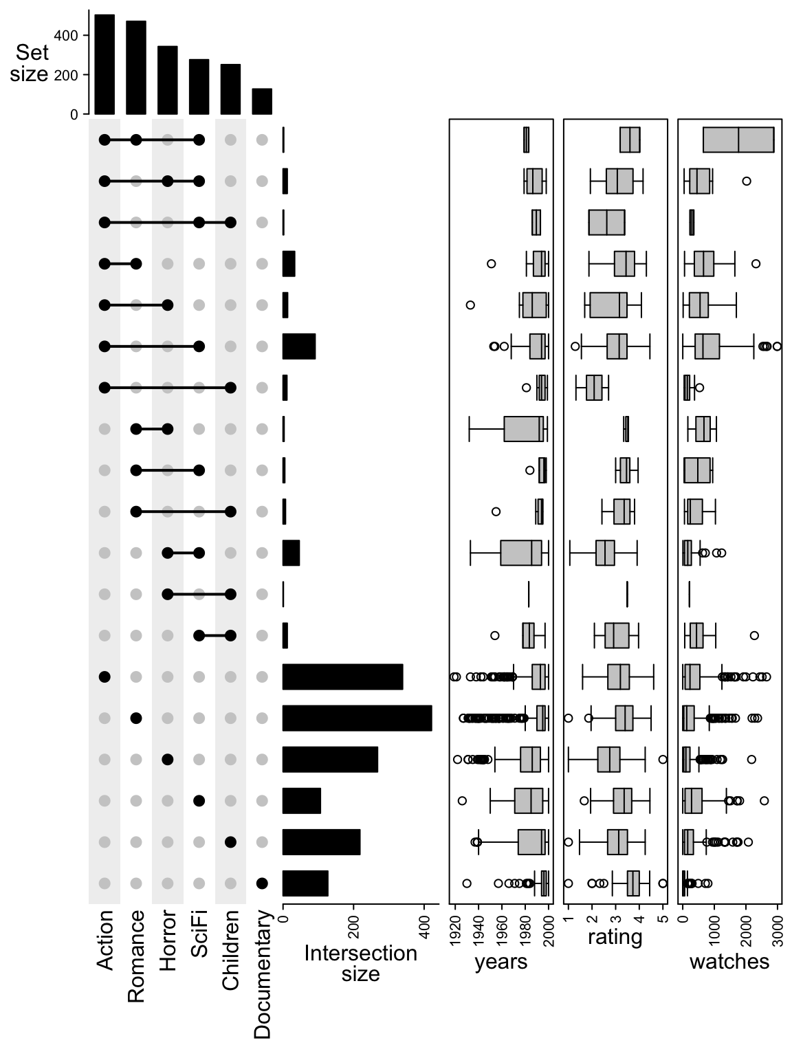
颠覆情节
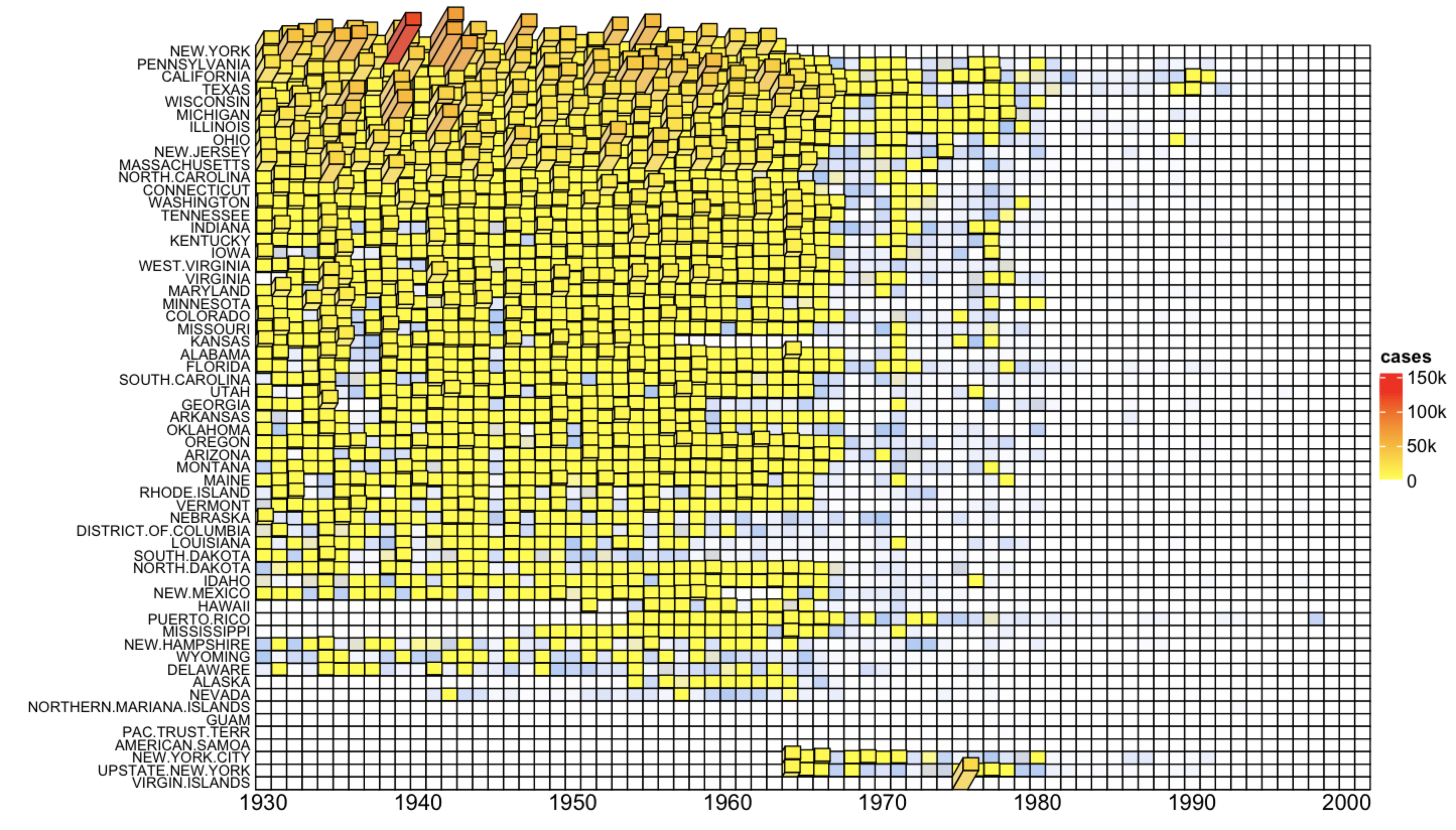
3D热图

🎨[可视化|R包]ComplexHeatmap学习笔记④Heatmap Annotations
Heatmap Annotations 热图注释
注释图形实际上非常普遍的。注释们的唯一共同特征是它们与热图的列或行对齐。这里有一个“HeatmapAnnotation”类,它用于定义列或行上的注释。
Column annotation 列注释
Simple annotation 简单注释
简单注释被定义为包含离散或连续值的向量。 由于简单注释被表示为向量,因此可以将多个简单注释指定为数据框(data frame)。 简单注释的颜色可以通过带有a vector或颜色映射函数的col指定,具体取决于简单注释是离散的还是连续的。
在热图中,简单的注释将被表示为网格行。.
HeatmapAnnotation类有一个draw()方法。 draw() is used internally and 在这里我们只是用它来演示。
library(ComplexHeatmap)
library(circlize)

df = data.frame(type = c(rep("a", 5), rep("b", 5)))
ha = HeatmapAnnotation(df = df)
ha
## A HeatmapAnnotation object with 1 annotation.
##
## An annotation with discrete color mapping
## name: type
## position: column
## show legend: TRUE
draw(ha, 1:10)
简单注释draw
应将简单注释的颜色指定给一个具有名称的list(颜色list中的名称,它对应于数据框中的名称)(这里就是指以下示例中的type)【注:下方颜色list的a,对应于数据df里的a】。 每个颜色向量应该更好地具有名称以映射到注释的级别。--给注释自定义颜色
ha = HeatmapAnnotation(df = df, col = list(type = c("a" =  "red", "b" = "blue")))
ha
## A HeatmapAnnotation object with 1 annotation.
##
## An annotation with discrete color mapping
## name: type
## position: column
## show legend: TRUE
draw(ha, 1:10)
给注释自定义颜色
对于连续值的注释,颜色由颜色映射函数定义.
ha = HeatmapAnnotation(df = data.frame(age = sample(1:20, 10)),
    col = list(age = colorRamp2(c(0, 20), c("white", "red"))))
ha
## A HeatmapAnnotation object with 1 annotation.
##
## An annotation with continuous color mapping
## name: age
## position: column
## show legend: TRUE
draw(ha, 1:10)
连续值注释
NA的颜色可以由na_col设置:
df2 = data.frame(type = c(rep("a", 5), rep("b", 5)),
                age = sample(1:20, 10))
df2$type[5] = NA
df2$age[5] = NA
ha = HeatmapAnnotation(df = df2,
  col = list(type = c("a" =  "red", "b" = "blue"),
             age = colorRamp2(c(0, 20), c("white", "red"))),
  na_col = "grey")
draw(ha, 1:10)
NA颜色设置
在数据框(data frame)中放置多个注释。.
df = data.frame(type = c(rep("a", 5), rep("b", 5)),
                age = sample(1:20, 10))
ha = HeatmapAnnotation(df = df,
    col = list(type = c("a" = "red", "b" = "blue"),
               age = colorRamp2(c(0, 20), c("white", "red")))
)
ha
## A HeatmapAnnotation object with 2 annotations.
##
## An annotation with discrete color mapping
## name: type
## position: column
## show legend: TRUE
##
## An annotation with continuous color mapping
## name: age
## position: column
## show legend: TRUE
draw(ha, 1:10)
多个注释
Also individual annotations can be directly specified as vectors:
ha = HeatmapAnnotation(type = c(rep("a", 5), rep("b", 5)),
                       age = sample(1:20, 10),
    col = list(type = c("a" = "red", "b" = "blue"),
               age = colorRamp2(c(0, 20), c("white", "red")))
)
ha
## A HeatmapAnnotation object with 2 annotations.
##
## An annotation with discrete color mapping
## name: type
## position: column
## show legend: TRUE
##
## An annotation with continuous color mapping
## name: age
## position: column
## show legend: TRUE
draw(ha, 1:10)
注释
要将列注释放到heatmap中,请在heatmap()中指定top_annotation和bottom_annotation.
ha1 = HeatmapAnnotation(df = df,
    col = list(type = c("a" = "red", "b" = "blue"),
               age = colorRamp2(c(0, 20), c("white", "red")))
)
ha2 = HeatmapAnnotation(df = data.frame(age = sample(1:20, 10)),
    col = list(age = colorRamp2(c(0, 20), c("white", "red"))))

set.seed(123)
mat = matrix(rnorm(80, 2), 8, 10)
mat = rbind(mat, matrix(rnorm(40, -2), 4, 10))
rownames(mat) = paste0("R", 1:12)
colnames(mat) = paste0("C", 1:10)

Heatmap(mat, top_annotation = ha1, bottom_annotation = ha2)
列注释
Complex annotations 复杂的注释
除了简单的注释,还有复杂的注释。复杂的注释总是被表示为自定义的图形函数。实际上,对于每个列注释, there will be a viewport created waiting for graphics。这里的注释函数定义了如何将图形放到这个viewport中。函数的唯一参数是列的索引,该索引是已经通过列聚类进行了调整的列索引 .
在下方的例子中, 将创建点的注释,请注意我们如何定义xscale,以便如果将注释添加到heatmap中,点的位置对应于列的中点.
value = rnorm(10)
column_anno = function(index) {
    n = length(index)
    # since middle of columns are in 1, 2, ..., n and each column has width 1
    # then the most left should be 1 - 0.5 and the most right should be n + 0.5
    pushViewport(viewport(xscale = c(0.5, n + 0.5), yscale = range(value)))
    # since order of columns will be adjusted by clustering, here we also
    # need to change the order by `[index]`
    grid.points(index, value[index], pch = 16, default.unit = "native")
    # this is very important in order not to mess up the layout
    upViewport()
}
ha = HeatmapAnnotation(points = column_anno)  # here the name is arbitrary
ha
## A HeatmapAnnotation object with 1 annotation.
##
## An annotation with self-defined function
## name: points
## position: column
draw(ha, 1:10)
点注释
以上代码仅用于演示。你不需要自己定义一个点注释,包中已经提供了几个注释生成器,如anno_points()或anno_barplot(),它们可以生成这些复杂的注释函数:
anno_points()anno_barplot()anno_boxplot()anno_histogram()anno_density()anno_text()
这些 anno_* 函数的输入值很简单. 可以是数值向量(e.g. for anno_points() and anno_barplot()), a matrix or list (for anno_boxplot(), anno_histogram() or anno_density()), or a character vector (for anno_text()).
ha = HeatmapAnnotation(points = anno_points(value))
draw(ha, 1:10)
anno_points
ha = HeatmapAnnotation(barplot = anno_barplot(value))
draw(ha, 1:10)
anno_barplot
anno_boxplot() 为矩阵中的每一列生成箱线图。.
ha = HeatmapAnnotation(boxplot = anno_boxplot(mat))
draw(ha, 1:10)
anno_boxplot
您可以混合使用简单注释和复杂注释:
ha = HeatmapAnnotation(df = df,
                       points = anno_points(value),
    col = list(type = c("a" = "red", "b" = "blue"),
               age = colorRamp2(c(0, 20), c("white", "red"))))
ha
## A HeatmapAnnotation object with 3 annotations.
##
## An annotation with discrete color mapping
## name: type
## position: column
## show legend: TRUE
##
## An annotation with continuous color mapping
## name: age
## position: column
## show legend: TRUE
##
## An annotation with self-defined function
## name: points
## position: column
draw(ha, 1:10)
混合使用简单注释和复杂注释
由于简单的注释也可以指定为向量,所以实际上可以按任意顺序排列注释:
ha = HeatmapAnnotation(type = c(rep("a", 5), rep("b", 5)),
                       points = anno_points(value),
                       age = sample(1:20, 10),
                       bars = anno_barplot(value),
    col = list(type = c("a" = "red", "b" = "blue"),
               age = colorRamp2(c(0, 20), c("white", "red"))))
ha
## A HeatmapAnnotation object with 4 annotations.
##
## An annotation with discrete color mapping
## name: type
## position: column
## show legend: TRUE
##
## An annotation with self-defined function
## name: points
## position: column
##
## An annotation with continuous color mapping
## name: age
## position: column
## show legend: TRUE
##
## An annotation with self-defined function
## name: bars
## position: column
draw(ha, 1:10)
任意顺序排列注释
对于一些 anno_*函数, 图形参数可以由gp设置. 也请注意我们如何在anno_barplot()中指定 baseline(基线).
ha = HeatmapAnnotation(barplot1 = anno_barplot(value, baseline = 0, gp = gpar(fill = ifelse(value > 0, "red", "green"))),
                       points = anno_points(value, gp = gpar(col = rep(1:2, 5))),
                       barplot2 = anno_barplot(value, gp = gpar(fill = rep(3:4, 5))))
ha
## A HeatmapAnnotation object with 3 annotations.
##
## An annotation with self-defined function
## name: barplot1
## position: column
##
## An annotation with self-defined function
## name: points
## position: column
##
## An annotation with self-defined function
## name: barplot2
## position: column
draw(ha, 1:10)
用gp设置
如果有多个注释,可以通过annotation_height控制每个注释的高度。annotation_height的值可以是数值,也可以是unit对象.
# set annotation height as relative values
ha = HeatmapAnnotation(df = df, points = anno_points(value), boxplot = anno_boxplot(mat),
    col = list(type = c("a" = "red", "b" = "blue"),
               age = colorRamp2(c(0, 20), c("white", "red"))),
    annotation_height = c(1, 2, 3, 4))
draw(ha, 1:10)
用数值设置注释高度
# set annotation height as absolute units
ha = HeatmapAnnotation(df = df, points = anno_points(value), boxplot = anno_boxplot(mat),
    col = list(type = c("a" = "red", "b" = "blue"),
               age = colorRamp2(c(0, 20), c("white", "red"))),
    annotation_height = unit.c((unit(1, "npc") - unit(4, "cm"))*0.5, (unit(1, "npc") - unit(4, "cm"))*0.5,
        unit(2, "cm"), unit(2, "cm")))
draw(ha, 1:10)
用unit对象设置数值高度
构造好注释后,您可以通过top_annotation或bottom_annotation来分配热图注释的位置。如果注释的高度是相对值,你还可以通过top_annotation_height和bottom_annotation_height来控制列注释的大小.
如果注释具有合适的大小(足够高),则在其上添加坐标轴(axis)将很有帮助。anno_points()、anno_barplot()和anno_boxplot()都支持坐标轴。请注意,我们没有为坐标轴预先分配空间,我们只是假设已经有空的空间来显示坐标轴.
ha = HeatmapAnnotation(df = df, points = anno_points(value),
    col = list(type = c("a" = "red", "b" = "blue"),
               age = colorRamp2(c(0, 20), c("white", "red"))))
ha_boxplot = HeatmapAnnotation(boxplot = anno_boxplot(mat, axis = TRUE))
Heatmap(mat, name = "foo", top_annotation = ha, bottom_annotation = ha_boxplot,
    bottom_annotation_height = unit(3, "cm"))
boxplot添加坐标轴
每个注释下面的间隔可以通过"HeatmapAnnotation()"中的"gap"来指定Gaps below each annotation can be specified by gap in HeatmapAnnotation().
ha = HeatmapAnnotation(df = df, points = anno_points(value), gap = unit(c(2, 4), "mm"),
    col = list(type = c("a" = "red", "b" = "blue"),
               age = colorRamp2(c(0, 20), c("white", "red"))))
Heatmap(mat, name = "foo", top_annotation = ha)
注释间添加间隔
在创建HeatmapAnnotation对象时,可以通过将show_legend指定为“FALSE”来禁止某些注释图例
ha = HeatmapAnnotation(df = df, show_legend = c(FALSE, TRUE),
    col = list(type = c("a" = "red", "b" = "blue"),
               age = colorRamp2(c(0, 20), c("white", "red"))))
Heatmap(mat, name = "foo", top_annotation = ha)
指定一些注释不显示
anno_histogram()和anno_density()支持更多类型的注释,这些注释显示在相应的列中数据分布.
ha_mix_top = HeatmapAnnotation(histogram = anno_histogram(mat, gp = gpar(fill = rep(2:3, each = 5))),
    density_line = anno_density(mat, type = "line", gp = gpar(col = rep(2:3, each = 5))),
    violin = anno_density(mat, type = "violin", gp = gpar(fill = rep(2:3, each = 5))),
    heatmap = anno_density(mat, type = "heatmap"))
Heatmap(mat, name = "foo", top_annotation = ha_mix_top, top_annotation_height = unit(8, "cm"))
注释:可展示数据分布
文本也是注释图形的一种。anno_text()支持添加文本作为热图注释。 使用此注释函数,可以轻松地使用旋转来模拟列名称。 请注意,您需要手动计算文本注释的空间,并且包不能保证所有旋转的文本都显示在图中(在下图中,如果不绘制行名称和图例,'C10C10C10'将被完全显示 ,一些使用技巧你可以在[** Examples **]vignette中找到.
long_cn = do.call("paste0", rep(list(colnames(mat)), 3))  # just to construct long text
ha_rot_cn = HeatmapAnnotation(text = anno_text(long_cn, rot = 45, just = "left", offset = unit(2, "mm")))
Heatmap(mat, name = "foo", top_annotation = ha_rot_cn, top_annotation_height = unit(2, "cm"))
文本注释
Row annotations 行注释
行注释也由HeatmapAnnotation class定义,但是需要将Row赋给which
df = data.frame(type = c(rep("a", 6), rep("b", 6)))
ha = HeatmapAnnotation(df = df, col = list(type = c("a" = "red", "b" = "blue")),
    which = "row", width = unit(1, "cm"))
draw(ha, 1:12)
行注释
有一个叫做rowAnnotation()的函数可以实现HeatmapAnnotation(..., which = "row")相同的功能.
ha = rowAnnotation(df = df, col = list(type = c("a" = "red", "b" = "blue")), width = unit(1, "cm"))
anno_* 含住在 row annotations中也同样有效,不过你需要给函数添加which = "row"参数. 例如:
ha = rowAnnotation(points = anno_points(runif(10), which = "row"))
与rowAnnotation()类似, there are corresponding wrapper anno_* functions. 除了预先定义的' which '参数到' row '之外,函数几乎与原始函数相同:
row_anno_points()row_anno_barplot()row_anno_boxplot()row_anno_histogram()row_anno_density()row_anno_text()
类似地,可以有多个行注释.
ha_combined = rowAnnotation(df = df, boxplot = row_anno_boxplot(mat),
    col = list(type = c("a" = "red", "b" = "blue")),
    annotation_width = c(1, 3))
draw(ha_combined, 1:12)
多个行注释
Mix heatmaps and row annotations 混合热图和行注释
从本质上讲,行注释和列注释是相同的图形,但在实践中有一些区别. 在ComplexHeatmap包中, 行注释与热图具有相同的地位,而列注释就像热图的附属组件。有这样的看法是因为行注释可以对应于列表中的所有热图,而列注释只能对应于它自己的热图。类似于heatmap,对于行注释,您可以将行注释附加到heatmap或heatmap列表,甚至行注释对象本身。行注释中的元素顺序也可以通过热图的聚类进行调整.
ha = rowAnnotation(df = df, col = list(type = c("a" = "red", "b" = "blue")),
    width = unit(1, "cm"))
ht1 = Heatmap(mat, name = "ht1")
ht2 = Heatmap(mat, name = "ht2")
ht1 + ha + ht2
行注释
如果再在热图中设置了 km 或 split, 行注释也将陪同被拆分.
ht1 = Heatmap(mat, name = "ht1", km = 2)
ha = rowAnnotation(df = df, col = list(type = c("a" = "red", "b" = "blue")),
    boxplot = row_anno_boxplot(mat, axis = TRUE),
    annotation_width = unit(c(1, 5), "cm"))
ha + ht1
行注释和主热图聚类对应:你拆分,我也跟着拆
当应用行分割时,graphical parameters for annotation function can be specified as with the same length as the number of row slices.
ha = rowAnnotation(boxplot = row_anno_boxplot(mat, gp = gpar(fill = c("red", "blue"))),
    width = unit(2, "cm"))
ha + ht1
由于只保留主热图的行聚类和行标题,因此可以通过设置row_hclust_side and row_sub_title_side将它们调整到图的最左边或右边:
draw(ha + ht1, row_dend_side = "left", row_sub_title_side = "right")
设置标题位置
Self define row annotations 自定义行注释
If row annotations are split by rows, the argument index will automatically be the index in the 'current' row slice.自定义行注释与自定义列注释相同。 唯一的区别是切换了x坐标和y坐标。 如果行注释按行分割,则参数 index 将自动成为'current'行切片中的索引。
value = rowMeans(mat)
row_anno = function(index) {
    n = length(index)
    pushViewport(viewport(xscale = range(value), yscale = c(0.5, n + 0.5)))
    grid.rect()
    # recall row order will be adjusted, here we specify `value[index]`
    grid.points(value[index], seq_along(index), pch = 16, default.unit = "native")
    upViewport()
}
ha = rowAnnotation(points = row_anno, width = unit(1, "cm"))
ht1 + ha
自定义行注释
对于自定义的注释函数,也可以有第二个参数“k”,它提供出“current”行切片的索引。.
row_anno = function(index, k) {
    n = length(index)
    col = c("blue", "red")[k]
    pushViewport(viewport(xscale = range(value), yscale = c(0.5, n + 0.5)))
    grid.rect()
    grid.points(value[index], seq_along(index), pch = 16, default.unit = "native", gp = gpar(col = col))
    upViewport()
}
ha = rowAnnotation(points = row_anno, width = unit(1, "cm"))
ht1 + ha
自定义行注释
Heatmap with zero row 零行的热图
如果只想可视化矩阵的元数据(meta data),你可以设置矩阵的行数为零。在这种情况下,只允许是一个热图(In this case, only one heatmap is allowed.)
ha = HeatmapAnnotation(df = data.frame(value = runif(10), type = rep(letters[1:2], 5)),
    barplot = anno_barplot(runif(10)),
    points = anno_points(runif(10)))
zero_row_mat = matrix(nrow = 0, ncol = 10)
colnames(zero_row_mat) = letters[1:10]
Heatmap(zero_row_mat, top_annotation = ha, column_title = "only annotations")
零行热图
如果您想比较多个指标(metrics),这个特性非常有用。下图中的坐标轴和标签由[heatmap decoration]添加。还请注意,我们是如何调整绘图区域的,以便为hte坐标轴标签提供足够的空间。
ha = HeatmapAnnotation(df = data.frame(value = runif(10), type = rep(letters[1:2], 5)),
    barplot = anno_barplot(runif(10), axis = TRUE),
    points = anno_points(runif(10), axis = TRUE),
    annotation_height = unit(c(0.5, 0.5, 4, 4), "cm"))
zero_row_mat = matrix(nrow = 0, ncol = 10)
colnames(zero_row_mat) = letters[1:10]
ht = Heatmap(zero_row_mat, top_annotation = ha, column_title = "only annotations")
draw(ht, padding = unit(c(2, 20, 2, 2), "mm"))
decorate_annotation("value", {grid.text("value", unit(-2, "mm"), just = "right")})
decorate_annotation("type", {grid.text("type", unit(-2, "mm"), just = "right")})
decorate_annotation("barplot", {
    grid.text("barplot", unit(-10, "mm"), just = "bottom", rot = 90)
    grid.lines(c(0, 1), unit(c(0.2, 0.2), "native"), gp = gpar(lty = 2, col = "blue"))
})
decorate_annotation("points", {
    grid.text("points", unit(-10, "mm"), just = "bottom", rot = 90)
})
image.png
Heatmap with zero column 零列的热图
如果不需要绘制热图,而用户只想要行注释列表,则可以将没有列的空矩阵添加到热图列表中。在零列矩阵中,可以拆分行注释:
ha_boxplot = rowAnnotation(boxplot = row_anno_boxplot(mat), width = unit(3, "cm"))
ha = rowAnnotation(df = df, col = list(type = c("a" = "red", "b" = "blue")), width = unit(2, "cm"))
text = paste0("row", seq_len(nrow(mat)))
ha_text = rowAnnotation(text = row_anno_text(text), width = max_text_width(text))
nr = nrow(mat)
Heatmap(matrix(nrow = nr, ncol = 0), split = sample(c("A", "B"), nr, replace = TRUE)) +
    ha_boxplot + ha + ha_text
零列注释
或将树图添加到行注释中:
dend = hclust(dist(mat))
Heatmap(matrix(nrow = nr, ncol = 0), cluster_rows = dend) +
    ha_boxplot + ha + ha_text
将树状图添加到行注释中
请记住,不允许只使用concantenate(串联)行注释,因为行注释并不提供行数信息
Use heatmap instead of simple row annotations 使用热图而不是简单的行注释
最后,如果您的行注释是简单的注释,我建议使用heatmap。以下两种方法可以生成类似的图形。
df = data.frame(type = c(rep("a", 6), rep("b", 6)))
Heatmap(mat) + rowAnnotation(df = df, col = list(type = c("a" = "red", "b" = "blue")),
    width = unit(1, "cm"))
简单行注释
Heatmap(mat) + Heatmap(df, name = "type", col = c("a" = "red", "b" = "blue"),
    width = unit(1, "cm"))
简单行注释
Axes for annotations 注释的坐标轴
对于复杂的注释,坐标轴对于显示数据的范围和方向非常重要。anno_*函数提供axis and axis_side参数来控制坐标轴.
ha1 = HeatmapAnnotation(b1 = anno_boxplot(mat, axis = TRUE),
    p1 = anno_points(colMeans(mat), axis = TRUE))
ha2 = rowAnnotation(b2 = row_anno_boxplot(mat, axis = TRUE),
    p2 = row_anno_points(rowMeans(mat), axis = TRUE), width = unit(2, "cm"))
Heatmap(mat, top_annotation = ha1, top_annotation_height = unit(2, "cm")) + ha2
注释坐标轴设置
对于行注释,数据的默认方向是从左到右。但是,如果将行注释放在heatmap的左侧,可能会让人感到困惑。您可以通过axis_direction更改行注释的坐标轴方向。比较以下两个图:
pushViewport(viewport(layout = grid.layout(nr = 1, nc = 2)))
pushViewport(viewport(layout.pos.row = 1, layout.pos.col = 1))
ha = rowAnnotation(boxplot = row_anno_boxplot(mat, axis = TRUE), width = unit(3, "cm"))
ht_list = ha + Heatmap(mat)
draw(ht_list, column_title = "normal axis direction", newpage = FALSE)
upViewport()

pushViewport(viewport(layout.pos.row = 1, layout.pos.col = 2))
ha = rowAnnotation(boxplot = row_anno_boxplot(mat, axis = TRUE, axis_direction = "reverse"),
    width = unit(3, "cm"))
ht_list = ha + Heatmap(mat)
draw(ht_list, column_title = "reverse axis direction", newpage = FALSE)
upViewport(2)
行注释坐标轴方向
Stacked barplots 堆叠barplots
如果输入是列大于1的矩阵,则Barplot注释可以是堆积条形图。 在这种情况下,如果将图形参数指定为向量,则其长度只能是1或者矩阵的列数。 由于条形图是堆叠的,因此每行只能包含所有正值或所有负值。
注意,缺点是对于堆叠的barplot没有图例,您需要手动生成它(检查[本节])
请注意,堆积条形图的缺点是没有图例,您需要手动生成它(请参阅 [this section])
foo1 = matrix(abs(rnorm(20)), ncol = 2)
foo1[1, ] = -foo1[1, ]
column_ha = HeatmapAnnotation(foo1 = anno_barplot(foo1, axis = TRUE))
foo2 = matrix(abs(rnorm(24)), ncol = 2)
row_ha = rowAnnotation(foo2 = row_anno_barplot(foo2, axis = TRUE, axis_side = "top",
    gp = gpar(fill = c("red", "blue"))), width = unit(2, "cm"))
Heatmap(mat, top_annotation = column_ha, top_annotation_height = unit(2, "cm"), km = 2) + row_ha
barplot注释堆叠
Add annotation names 添加注释名
从版本1.11.5开始,HeatmapAnnotation() 支持将注释名称直接添加到注释中。 但是,由于包的设计,有时名称将位于图形之外或与其他热图组件重叠,因此,默认情况下它将被关闭.
df = data.frame(type = c(rep("a", 5), rep("b", 5)),
                age = sample(1:20, 10))
value = rnorm(10)
ha = HeatmapAnnotation(df = df, points = anno_points(value, axis = TRUE),
    col = list(type = c("a" = "red", "b" = "blue"),
               age = colorRamp2(c(0, 20), c("white", "red"))),
    annotation_height = unit(c(0.5, 0.5, 2), "cm"),
    show_annotation_name = TRUE,
    annotation_name_offset = unit(2, "mm"),
    annotation_name_rot = c(0, 0, 90))
Heatmap(mat, name = "foo", top_annotation = ha)
给注释添加名称
Or the row annotation names:注意我们手动调整padding以完全显示points的文本。
df = data.frame(type = c(rep("a", 6), rep("b", 6)),
                age = sample(1:20, 12))
value = rnorm(12)
ha = rowAnnotation(df = df, points = row_anno_points(value, axis = TRUE),
    col = list(type = c("a" = "red", "b" = "blue"),
               age = colorRamp2(c(0, 20), c("white", "red"))),
    annotation_width = unit(c(0.5, 0.5, 2), "cm"),
    show_annotation_name = c(TRUE, FALSE, TRUE),
    annotation_name_offset = unit(c(2, 2, 8), "mm"),
    annotation_name_rot = c(90, 90, 0))
ht = Heatmap(mat, name = "foo") + ha
draw(ht, padding = unit(c(4, 2, 2, 2), "mm"))
Adjust positions of column names 或者行注释名称:注意我们手动调整padding以完全显示“points”的文本。
在热图组件的布局中,列名称直接放在热图主体下方。 当注释放在热图的底部时,这将导致问题:--注意列名和列注释的位置
ha = HeatmapAnnotation(type = df$type,
    col = list(type = c("a" = "red", "b" = "blue")))
Heatmap(mat, bottom_annotation = ha)
为了解决这个问题,我们可以用文本注释替换列名。
ha = HeatmapAnnotation(type = df$type,
    colname = anno_text(colnames(mat), rot = 90, just = "right", offset = unit(1, "npc") - unit(2, "mm")),
    col = list(type = c("a" = "red", "b" = "blue")),
    annotation_height = unit.c(unit(5, "mm"), max_text_width(colnames(mat)) + unit(2, "mm")))
Heatmap(mat, show_column_names = FALSE, bottom_annotation = ha)
列名用文本注释来弄
添加文本注释时,应计算文本的最大宽度并将其设置为文本注释viewport的高度,以便所有文本都可以在图中完全显示。 有时,您还需要设置rot,just和offset以将文本与正确的锚位置对齐。.
Mark some of the rows/columns 标记一些行列
从版本1.8.0开始,添加了一个新的注释函数anno_link(),它通过链接连接标签和行的子集。 当有许多行/列并且我们想要标记某些行时(例如在基因表达矩阵中,我们想要标记一些重要的感兴趣的基因),这是有帮助的。--标记特定行
mat = matrix(rnorm(10000), nr = 1000)
rownames(mat) = sprintf("%.2f", rowMeans(mat))
subset = sample(1000, 20)
labels = rownames(mat)[subset]
Heatmap(mat, show_row_names = FALSE, show_row_dend = FALSE, show_column_dend = FALSE) +
rowAnnotation(link = row_anno_link(at = subset, labels = labels),
  width = unit(1, "cm") + max_text_width(labels))
标记特定行
# here unit(1, "cm") is width of segments
还有两个快捷函数: row_anno_link() and column_anno_link().
Session info
sessionInfo()
## R version 3.5.1 Patched (2018-07-24 r75008)
## Platform: x86_64-w64-mingw32/x64 (64-bit)
## Running under: Windows Server 2012 R2 x64 (build 9600)
##
## Matrix products: default
##
## locale:
## [1] LC_COLLATE=C                           LC_CTYPE=English_United States.1252
## [3] LC_MONETARY=English_United States.1252 LC_NUMERIC=C
## [5] LC_TIME=English_United States.1252
##
## attached base packages:
##  [1] stats4    parallel  grid      stats     graphics  grDevices utils     datasets  methods
## [10] base
##
## other attached packages:
##  [1] dendextend_1.9.0      dendsort_0.3.3        cluster_2.0.7-1       IRanges_2.16.0
##  [5] S4Vectors_0.20.0      BiocGenerics_0.28.0   HilbertCurve_1.12.0   circlize_0.4.4
##  [9] ComplexHeatmap_1.20.0 knitr_1.20            markdown_0.8
##
## loaded via a namespace (and not attached):
##  [1] mclust_5.4.1           Rcpp_0.12.19           mvtnorm_1.0-8          lattice_0.20-35
##  [5] png_0.1-7              class_7.3-14           assertthat_0.2.0       mime_0.6
##  [9] R6_2.3.0               GenomeInfoDb_1.18.0    plyr_1.8.4             evaluate_0.12
## [13] ggplot2_3.1.0          highr_0.7              pillar_1.3.0           GlobalOptions_0.1.0
## [17] zlibbioc_1.28.0        rlang_0.3.0.1          lazyeval_0.2.1         diptest_0.75-7
## [21] kernlab_0.9-27         whisker_0.3-2          GetoptLong_0.1.7       stringr_1.3.1
## [25] RCurl_1.95-4.11        munsell_0.5.0          compiler_3.5.1         pkgconfig_2.0.2
## [29] shape_1.4.4            nnet_7.3-12            tidyselect_0.2.5       gridExtra_2.3
## [33] tibble_1.4.2           GenomeInfoDbData_1.2.0 viridisLite_0.3.0      crayon_1.3.4
## [37] dplyr_0.7.7            MASS_7.3-51            bitops_1.0-6           gtable_0.2.0
## [41] magrittr_1.5           scales_1.0.0           stringi_1.2.4          XVector_0.22.0
## [45] viridis_0.5.1          flexmix_2.3-14         bindrcpp_0.2.2         robustbase_0.93-3
## [49] fastcluster_1.1.25     HilbertVis_1.40.0      rjson_0.2.20           RColorBrewer_1.1-2
## [53] tools_3.5.1            fpc_2.1-11.1           glue_1.3.0             trimcluster_0.1-2.1
## [57] DEoptimR_1.0-8         purrr_0.2.5            colorspace_1.3-2       GenomicRanges_1.34.0
## [61] prabclus_2.2-6         bindr_0.1.1            modeltools_0.2-22


评论区